Simulating Connectomes with Claude Code

Connectomes give you the wiring diagram of a brain. Every neuron, every synapse, the exact count of connections between any two cells. The fly brain alone has 130,000 neurons and tens of millions of synapses, all mapped at nanometer resolution. The promise is that you can take this wiring, pour it into a simulation, and watch the circuit compute. The reality is that the connectome doesn't tell you how strong each synapse is, only how many there are, and the bhavior you get depends on biophysical parameters that have to come from somewhere else. Bhalla and Bower tried this for olfactory cortex thirty years ago. The field is still trying. But the datasets are newer, bigger, and more complete than anything that existed even five years ago, and there are a lot of people working on closing that gap.

I wanted to see what happens when you give an AI coding agent the full connectome of two fly navigation circuits, a spiking simulator (Brian2), and a well-defined scientific question. Claude Code querying real connectivity data through an MCP server I built for connectomics, building models at increasing levels of biological realism, and iterating on the results, not as a demo but as an actual attempt to do science.

I ran two projects this way using data from the FlyWire connectome. The first modeled the head direction ring attractor with 46 EPG compass neurons and 32 Delta7 inhibitory neurons, asking whether the real connectivity can sustain a stable heading bump in a spiking network. The second modeled 360-degree motor steering with ~24 PFL3 neurons that reading a heading signal, asking whether they produce the sinusoidal motor commands that existing rate models predict. Each project took roughly a day of intensive back-and-forth with Claude Code: prompting, debugging, reinterpreting results, hitting walls, and occasionally discovering that what looked like a result was actually an artifact.

This post is about what that process taught me. The scientific findings live in the supplement. Here, the story is about working with an AI that can run simulations and analyze data faster than I can, but that doesn't check the literature before building a theory, doesn't compute whether a parameter should work before trying it, and doesn't question its own results until I force it to. Over the course of these projects I wrote a Skill file encoding the methodology for this kind of simulation, and every section in it traces back to a specific mistake we made. But those mistakes were also what led to the science: the real fly connectome sustains a spiking ring attractor where idealized symmetric models can't, because the wiring heterogeneity that looks like noise in the diagram turns out to decorrelate neural activity in exactly the way the network needs. That's the kind of finding that falls out of taking real wiring seriously, and it's the kind of finding that a fast, sometimes reckless partner helps you stumble into sooner.

---

The head direction ring attractor

Claude Code pulled the FlyWire head direction circuit: 46 EPG neurons, 20 PEN1, 22 PEN2, 32 Delta7, totaling 5,049 edges and 165,484 synapses across 16 connection types. It analyzed the connectivity and identified the key pathways: EPG→EPG recurrence, the EPG→Delta7→EPG inhibitory loop, PEN→EPG velocity input. Standard ring attractor architecture, consistent with the literature.

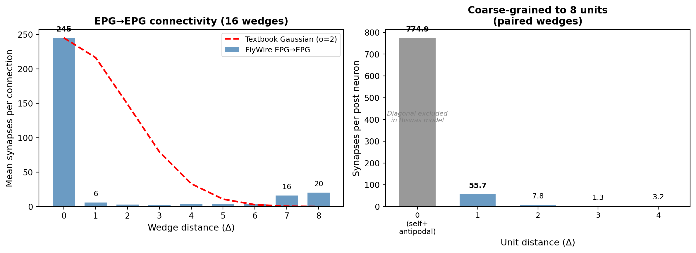
The first surprise was in the EPG→EPG connectivity profile. Textbook ring attractors use a smooth Gaussian or cosine excitatory profile: each neuron excites its neighbors, the excitation falls off with distance, and the result is a single smooth bump of activity. The real wiring looked nothing like that. At the level of individual EB wedges, EPG→EPG connections were almost entirely same-wedge: 245 synapses per connection at Δ0 versus 6 at Δ1 (averages across edges; total counts are 33,590 and 666 respectively), a 41:1 ratio. A second peak appeared at 7–8 wedges away, the antipodal position on the ring. After coarse-graining to the 8 computational units that theoretical models use (pairing wedges across the two PB hemispheres), those antipodal connections become same-unit connections and the effective nearest-neighbor coupling turns out to be significant. But we didn't know that yet. What we saw in the raw data was a connectivity profile with no obvious lateral spread.

CC built a spiking simulation using this connectivity and found two bumps of activity at antipodal positions on the ring. It flagged this as a problem: parasitic secondary activity that needed to be suppressed. I pushed back. The protocerebral bridge maps onto the ellipsoid body with a dual cover, each PB glomerulus mapping to two EB wedges 180° apart. Calcium imaging shows paired activity in the protocerebral bridge (left and right glomeruli for each heading), though the ellipsoid body itself shows a single bump. So paired activity in a PB-level simulation seemed consistent with the anatomy. CC re-analyzed its results under this interpretation and found that its supposedly broken result matched the paired structure. Then it went further than I intended: it proposed that Delta7 implements winner-take-all among 8 wedge-pairs rather than 16 individual wedges, and built out a full framework of discrete attractor dynamics with Delta7-mediated competition. I didn't propose the WTA interpretation. CC did, extrapolating from a more modest reframe I'd offered. But I accepted it, and we both spent considerable time developing it.

We were both wrong, though not about everything. The paired activity pattern is real, a consequence of the PB↔EB mapping. What was wrong was the discrete dynamics: the two bumps parking at fixed positions, the WTA competition between wedge-pairs. The Biswas framework, which we found only after a belated literature review, showed that the fix wasn't simply balancing excitation against inhibition. The double degeneracy conditions impose specific algebraic constraints on the spatial profile of the effective weight matrix so that the bump can sit at any position without drifting to a preferred location. Simple weight normalization, which CC tried extensively, can't achieve this. When CC implemented the Biswas rate model with gamma values satisfying these constraints, the continuous attractor emerged and the discrete parking positions disappeared.

The Skill file lesson: literature review is the first step, not a recovery step after you've built a theory. CC didn't search because it wasn't prompted to, and I didn't insist because we were making what felt like progress. The WTA framework was plausible, internally consistent, and supported by the simulation data. That's exactly the failure mode: when the AI constructs a coherent story from the data in front of it, there's no internal signal that the story is wrong. The external check has to come from the literature, and it has to come early.

From rate model to spiking network

The Biswas rate model gave us the correct weights. The next step was to see whether the continuous attractor survives the transition to spiking neurons. The standard approach is to coarse-grain first: group the 46 EPG neurons into 8 units of 5–6 neurons each, all sharing identical connectivity within a unit. Get the coarse-grained spiking model working, then move to per-neuron connectivity. Don't skip levels.

The coarse-grained model failed, and understanding why took most of the project.

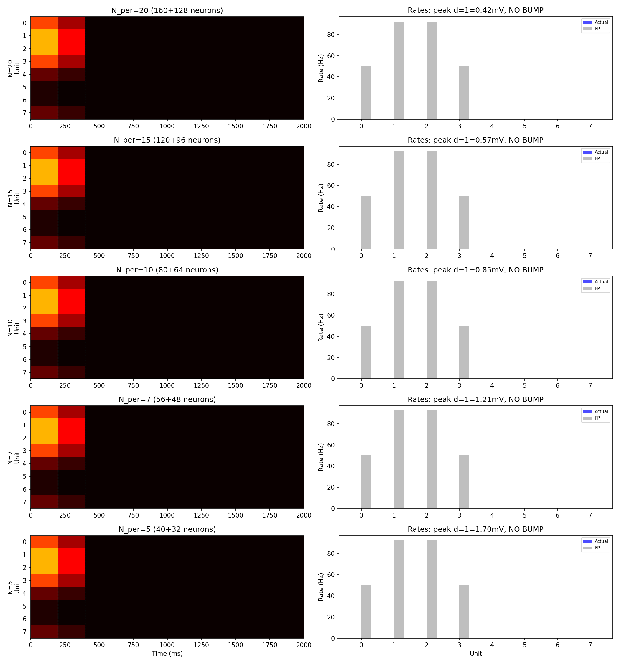
The Biswas rate model predicts what firing rate each unit should produce: high at the bump, near-zero away from it. The question is whether small groups of spiking neurons actually produce those rates. They don't, and the reason is structural. In the coarse-grained model, all 5–6 neurons within a unit share the same connectivity: the same presynaptic partners, the same synapse counts. They receive identical input, so they fire in near-synchrony. Their spikes arrive at downstream neurons in correlated clumps rather than spread out in time. Between clumps, the membrane voltage decays. The effective drive is lower than it would be if the same total number of spikes arrived independently, which is what the rate model assumes. The result: bump-position neurons fire at systematically lower rates than the rate model predicts, and the bump can't sustain itself.

CC confirmed this by running the simulation at population sizes from 5 to 20 neurons per unit: the bump died identically at every size, ruling out finite-size effects in one experiment. More neurons per unit doesn't help, because adding neurons with the same connectivity doesn't decorrelate anything. The correlation is structural.

We tried to compensate by improving the synapse model. Conductance-based synapses with alpha-shaped kinetics widen the margin between threshold and the resting voltage of off-bump neurons (from 2 mV to 17 mV through shunting), which helps suppress spurious firing away from the bump. But widening the margin doesn't fix the correlated-input problem at the bump itself. The bump still dies when external drive is removed.

Along the way, one of those failed coarse-grained simulations appeared to work. The bump formed, persisted for seconds after the drive was removed, and remained stable. We ran several analyses on top of it. Then CC tested what should have been a routine diagnostic: it forced a current injection into an off-bump unit and observed zero response. Investigation revealed that the voltage deflection for that unit was NaN. CC had computed initial currents using a function that returns NaN at zero firing rate, and Brian2 evaluates NaN > V_threshold as False, so those neurons had been permanently silent from the start. The bump was never self-sustaining. It was sustained by accidentally broken neurons that created artificial off-bump suppression. The NaN warning had been present in every previous run, but CC had suppressed it and I never saw it.

The Skill file lesson here is about methodology, not about NaN specifically. The perturbation test surfaced the bug because it forced the simulation into a region of state space we hadn't explored: what happens when you poke a unit that should be quiet? If we had only ever looked at the bump itself, we'd never have noticed. The general principle: probe your simulation across its state space, not just at the operating point you expect.

Why the real connectome works

CC built a spiking simulation using the actual per-neuron connectivity: all 46 EPG neurons with their individual synapse counts to each other and to the 32 Delta7 neurons, rather than grouping them into symmetric units. The synapse counts were scaled into synaptic conductances using the same pathway-level scaling factors from the rate model. Same neuron model, same synapse model. This didn't work on the first try: the scaling factors needed adjustment to account for the different number of presynaptic partners each neuron has in the full network, and early attempts produced either uniform saturation or complete silence. But CC had learned from the coarse-grained failures what the right parameter regime looked like, and after a targeted scan, the bump self-sustained.

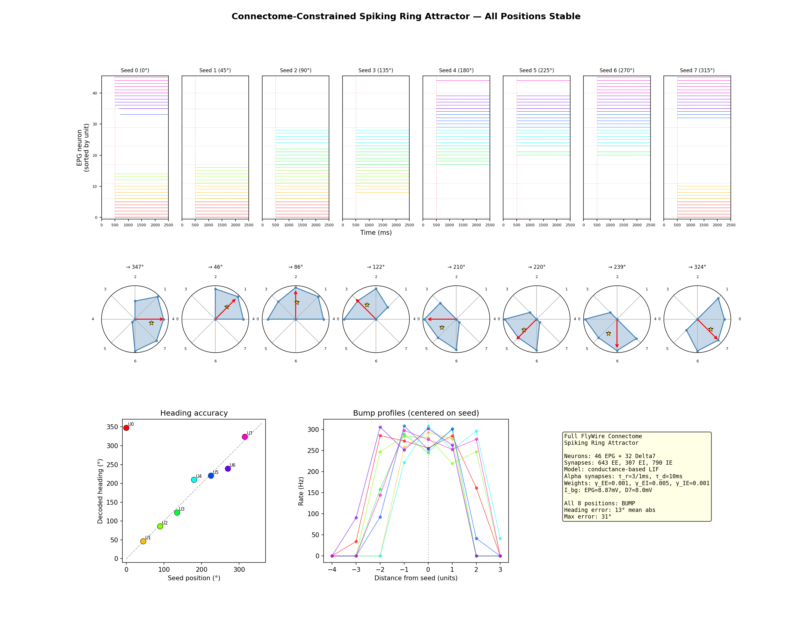
All 8 ring positions stable. The bump persisted for 3+ seconds after the seed was withdrawn. Firing rates of 250–300 Hz with clear spatial structure: 4–6 active units, 2–4 silent. These rates are higher than physiological EPG rates from electrophysiology (typically 20–80 Hz), likely reflecting the simplified biophysics of the LIF model and the absence of neuromodulatory tone. The decoded heading tracked the seed position with 13° mean error.

Why it works: each EPG neuron has a slightly different set of synapse counts to its partners. Neurons within the same wedge no longer receive identical input. Their spike times decorrelate. The postsynaptic neurons see input that's spread out in time rather than arriving in clumps, and the effective drive matches the rate model prediction. The heterogeneous connectivity does exactly what the symmetric model couldn't: it breaks the spike-time correlations that suppress firing rates below the self-sustaining threshold.

This is the result I find most interesting from the whole project. The theory knows that small identical-neuron networks produce discrete rather than continuous attractors, and addresses it through precise tuning of excitatory coupling (Noorman et al. 2024). The connectome solves the same problem differently: through heterogeneity. The wiring variability that looks like noise in the connectivity matrix decorrelates activity within each population in exactly the way the network needs. That's not something the theory predicts, and it only becomes visible when you simulate the real wiring at the single-neuron level.

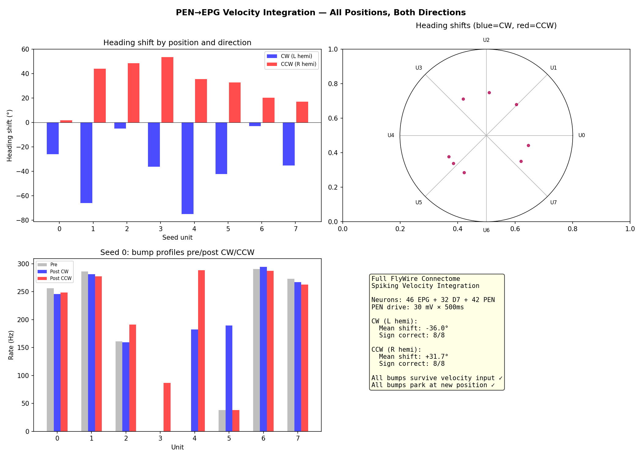
CC then added all 42 PEN neurons with their real PEN→EPG connectivity and tested velocity integration using spatially selective drive: direct current injection into PEN neurons within 2 positions of the bump, mimicking input that's already been gated to bump-adjacent neurons. This produced clean bidirectional translation (8/8 CW, 8/8 CCW), with the bump shifting and parking at the new position. The total heading shift varied dramatically across ring positions, from 3° to 75° for an identical stimulus, reflecting the heterogeneous distribution of PEN neurons across wedges. How the circuit achieves that spatial selectivity in vivo, rather than having it provided externally, remains open.

One additional finding: CC traced the velocity input pathway upstream of PEN and found that the signal arrives through GABAergic neurons providing hemisphere-specific tonic suppression. Velocity integration works by disinhibition: the velocity signal silences inhibitory neurons on one side, releasing PEN on that hemisphere. This confirmed that CW/CCW coding is hemisphere-selective (left PB = CW, right PB = CCW), not PEN1-vs-PEN2 as earlier models assumed.

---

The steering circuit

The head direction project ended with a working ring attractor and a methodology for getting there. The next question was whether the same approach could extend to a downstream circuit: one that reads the heading signal and converts it into motor commands. The PFL3 neurons do this. They receive input from the compass (EPG) neurons, and their output splits into two populations projecting to opposite sides of the lateral accessory lobe, a premotor area. The theoretical prediction, from models by Stone (2017) and Westeinde et al. (2024), is that PFL3 produces a sinusoidal steering signal: the difference in activity between the left-projecting and right-projecting populations varies as a sine function of the difference between the fly's current heading and its goal direction. Turn left when the goal is to the left, turn right when it's to the right, with the strength proportional to how far off-course you are.

What the connectome contains

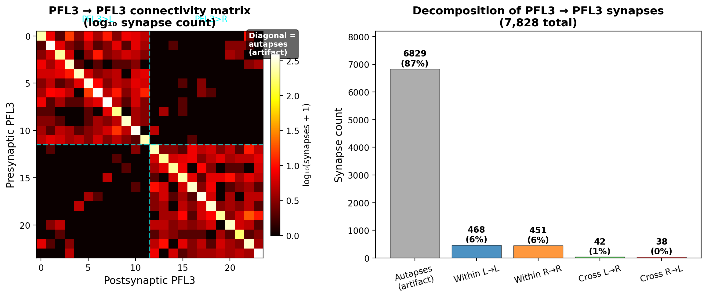
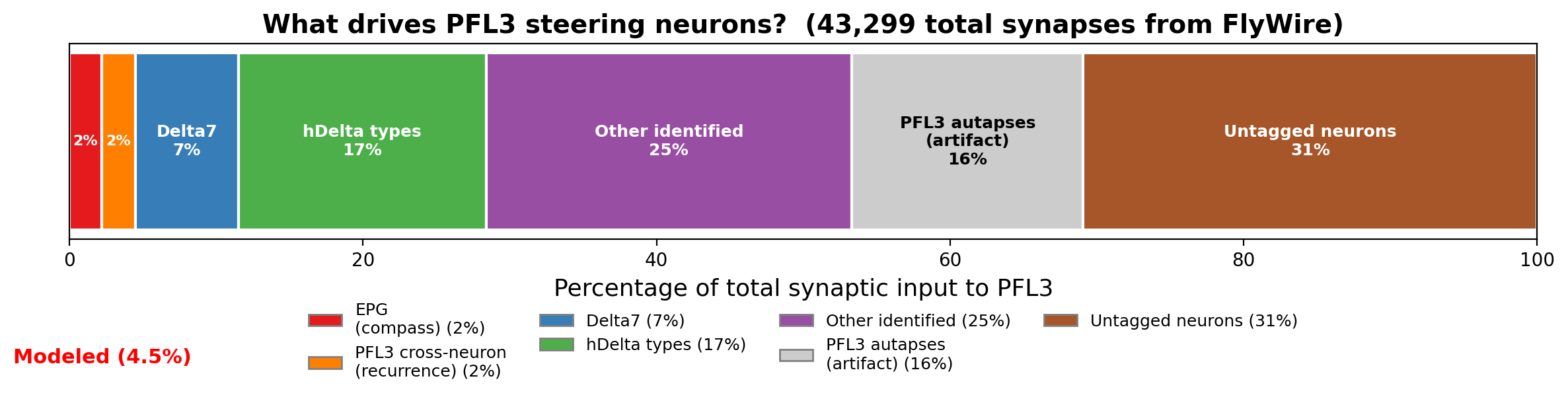
Existing models of PFL3 treat the compass neurons as the primary input driving the steering computation. The connectome tells a different story. EPG provides only 2% of PFL3's total synaptic input: 946 synapses out of roughly 43,000. Delta7 provides 7%, hDelta types provide 17%, and 31% is completely untagged. PFL3→PFL3 connections appeared to be the single largest identified input class at 18%, with 7,828 synapses. No existing model includes PFL3 recurrence.

The EPG→PFL3 wiring itself was clean but heterogeneous. Each PFL3 neuron has one dominant EPG column input (a clean diagonal in the connectivity matrix), but the weights vary roughly 7-fold across columns, with one column (L4) dramatically weak at 15 synapses versus a ~70 average. The push-pull output architecture was confirmed: right-heading PFL3 neurons project almost exclusively to one LAL output neuron, left-heading to the other, with ~200:1 segregation.

These numbers shaped what we built. The EPG pathway, despite being only 2% of total input, is the only heading-related input with a well-characterized computational role. So we modeled it as a null hypothesis: does this pathway alone, with the real synapse counts, produce the sinusoidal steering that theory predicts? And does the 18% recurrence change anything?

CC proposed following the standard abstraction ladder: build an idealized rate model first, then progressively add connectome features. I pushed for building two rate models in parallel instead: a textbook version with smooth sinusoidal connectivity and no recurrence as the null hypothesis, and a connectome-informed version using the real synapse counts. The differences between them are the science.

Both rate models produced highly sinusoidal steering curves (R² > 0.998), meaning the 7-fold weight variation across columns doesn't break the sinusoidal computation. Population averaging across ~12 neurons per side smooths it out. The connectome model produced half the steering amplitude of the textbook version (11.3 vs 21.3 Hz) and a -23° phase shift, both arising from the asymmetric EPG→PFL3 weights.

Then we tried to convert the rate model to a spiking simulation, and CC fell apart.

CC's spiral and the calibration protocol

CC spent over twenty minutes cycling through failed attempts, treating the conversion as a unit-scaling problem: searching for a single linear factor that would map rate model outputs to membrane voltages. Neurons saturated at 500 Hz or went completely silent, and CC adjusted one parameter at a time without a systematic framework. It mixed Brian2 unit systems with raw numpy, producing quantities in the wrong units. It lumped dozens of synapses into single connections, creating enormous per-spike transients. Each fix created a new problem.

The intervention was to impose a structured calibration protocol. Step 1: characterize the single LIF neuron's frequency-current curve analytically and verify it in Brian2. Step 2: derive the per-synapse weight from the f-I curve and the known presynaptic firing rate. Step 3: validate single-population dynamics without recurrence. Step 4: add recurrence. Step 5: compare against the rate model. Each step has a clear validation criterion, and you don't proceed until the current step matches its prediction. This is the kind of systematic reasoning CC should have done on its own. It didn't. It defaulted to guess-and-check because that's faster in the short term and it doesn't have the dynamical systems intuition to know where to start.

Once given the protocol, CC executed it cleanly. The f-I curve matched the analytical prediction, the per-synapse weight came out to 0.086 mV, and the single-population test matched the rate model with a mean error of 0.7 Hz across 24 neurons.

The Skill file lesson: form quantitative expectations before running a simulation. If you can't predict the order of magnitude of the firing rate, the synaptic weight, or the voltage response, you don't understand the model well enough to debug it. CC can run a simulation in seconds, which makes guess-and-check tempting. But each failed guess generates data that has to be interpreted, and interpreting wrong results takes longer than deriving the right answer analytically.

What spiking dynamics reveal

The spiking model with calibrated weights produced a steering curve that was still sinusoidal (R² = 0.992) with reduced amplitude (7.0 Hz versus 11.3 Hz in the rate model, 21.3 Hz in the textbook). The amplitude reduction comes from spike noise and refractoriness. The -23° phase shift from asymmetric weights was partially preserved (-14.9°): noise washed out some but not all of the structural asymmetry.

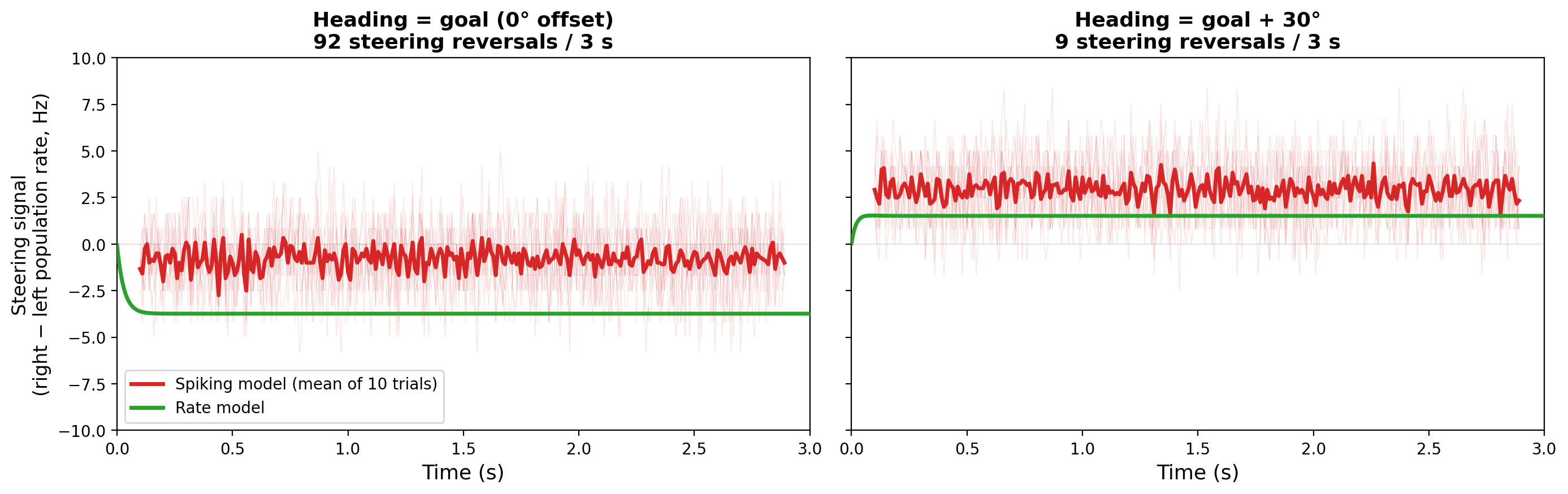
The spiking-specific finding was near-goal flickering. When the fly's heading is close to its goal (within about ±10°), the steering signal flickers rapidly between "turn left" and "turn right": 91 sign changes in 3 seconds at 0° heading-goal offset, compared to 3–22 sign changes at ±30° offset. The rate model predicts smooth convergence to zero at heading = goal. The spiking model says the signal is incoherent there. This defines an angular dead zone where PFL3 can't maintain a consistent steering direction, set by the population size (~12 neurons per side). It's a shot-noise effect: with so few neurons, the random timing of individual spikes dominates the population average when the true signal is near zero.

The autapse catch

With 18% of PFL3's input apparently coming from other PFL3 neurons, recurrence should matter. It could amplify the steering signal, sharpen the transition into and out of the dead zone, or create winner-take-all dynamics that lock in a turning direction near goal. Any of these would visibly change the flickering behavior. But when CC varied the recurrence strength from 0× to 1× of its biophysically derived value, the flickering was essentially unchanged. 18% of a neuron's input doing nothing to its dynamics is strange.

CC decomposed the recurrent input analytically and found the answer: 87% of recurrent synapses were self-connections. Neuron A synapsing onto itself. The resulting postsynaptic voltage deflection was 24.6 mV per spike. CC built a detailed mechanistic interpretation around this: recurrence provides persistence (each neuron reinforces its own activity) without competition (self-connections don't couple different neurons), explaining why it doesn't affect population-level dynamics like the flickering.

The interpretation was wrong, and there were two independent reasons CC should have caught it. The first is biophysical: a 24.6 mV voltage deflection from a single self-synapse is larger than the gap between threshold and rest. One spike would guarantee the neuron's own immediate re-firing, which no real neuron does. That's a sanity check CC could have run without any specialized knowledge. The second requires domain expertise: self-connections in Drosophila neurons (autapses) are a known artifact of automated synapse detection in connectome reconstructions. The segmentation algorithm occasionally assigns a presynaptic and postsynaptic site to the same neuron when they belong to different neurons passing close together. Biologically, autapses are essentially absent in the fly.

I caught the autapse artifact from experience with connectome data. CC had analyzed the data correctly, built an internally consistent story, and never questioned whether the data itself was real. The 87% figure, the 24.6 mV self-PSP, and the "persistence without competition" framework were all built on segmentation noise.

After removing autapses, corrected recurrence dropped to about 2% of total input, with a mean voltage deflection of 0.40 mV (2.5% of total drive). The results without recurrence — including the near-goal flickering — were now the most biologically relevant.

What we modeled and what we didn't

The autapse correction forced a broader accounting. The EPG pathway and the corrected recurrence together account for roughly 4% of PFL3's total synaptic input. Delta7 and hDelta types together provide 24%. Nearly a third is from neurons that haven't been assigned a cell type in FlyWire.

Some claims survive this accounting. The EPG pathway alone produces sinusoidal steering, robust to the 7-fold wiring heterogeneity across columns. Spiking dynamics introduce a precision limit near goal from population size: a dead zone exists. Genuine PFL3 recurrence is negligible. These don't depend on what the other 96% of input is doing.

Other claims need caveating: the absolute steering amplitude, the specific width of that dead zone, and the temporal dynamics could all change substantially when the unmodeled pathways are included.

But the unmodeled pathways aren't a dead end. They're a gradient of tractability. Delta7 is immediately modelable: its role is characterized, the wiring is mapped, and it's inhibitory and heading-tuned. Adding it could change the steering amplitude, sharpen tuning, or interact with the noise floor in ways that aren't obvious from the current model. The hDelta types require tracing their upstream inputs through the connectome to determine what signals they carry — nobody has done this systematically, so it's genuinely new science rather than implementing a known circuit. The 31% untagged neurons are the most uncertain, but "untagged" in FlyWire means lacking a cell-type label, not untraceable. Every one of those presynaptic neurons has a fully reconstructed morphology. Tracing their inputs and outputs to infer function is exactly the kind of discovery that connectomics enables, and the tools exist to do it.

---

What Claude Code does and what it doesn't

The pattern across both projects was consistent. CC was fast at pulling connectivity data, building simulations, running parameter sweeps, and generating diagnostic figures. When given a clear protocol, it executed reliably and quickly. It found relevant papers when asked to search. It characterized connectivity profiles, identified structural anomalies in the wiring, and produced quantitative analyses of its own simulation results.

What CC didn't do was the part of science that sits between the data and the interpretation. It didn't search the literature before building a theory. It didn't compute whether a parameter should work before trying it. It didn't notice that a 24.6 mV self-synapse is biologically impossible, or that its simulation was sustained by NaN-disabled neurons, or that the discrete attractor dynamics it found contradicted decades of calcium imaging data. Each of these required something different (domain knowledge, theoretical reasoning, basic sanity-checking), but they share a common structure: stepping back from the result in front of you and asking whether it makes sense in a larger context. CC doesn't do that unprompted. It treats each result as a starting point for the next action rather than as a claim to be interrogated.

The productive mode was a division of labor that emerged naturally over the two projects. I set the scientific direction, chose what to model, decided when to abandon an approach, and provided the skepticism when results seemed too clean or too strange. CC provided the implementation speed. What would take me a day of coding and debugging took minutes. The iteration cycle compressed dramatically. But the compression only helped when the direction was right, and setting the direction was always mine.

The Skill file came out of this. Every section in it addresses a specific failure: check the literature first, form quantitative predictions before simulating, validate across the state space, question connectome data quality, don't skip levels in the abstraction ladder. It's a document that encodes what I learned from working with CC, written so that CC can follow it on the next project. In a sense, it's a way of giving the AI the theoretical and methodological instincts it lacks: not by making it smarter, but by making the protocol explicit enough that it doesn't need to be.

Whether this scales beyond my specific use case, I'm not sure. The Skill file works because these two circuits are well-enough characterized that I could recognize when CC went wrong. For circuits where less is known — the hDelta inputs to PFL3, the untagged 31% — the human's ability to catch errors shrinks along with the available ground truth. The further you get from known biology, the more you depend on the AI's results being right, and these projects show exactly how much that dependence costs when the results are wrong.

What I'm left with is a way of working that I didn't have before. I can go from a connectome dataset to a spiking simulation in hours rather than days or weeks. The MCP server handles the data access, the Skill file handles the methodology, and CC handles the implementation. The science — the interpretation, the skepticism, the judgment calls — is still mine. For now, that division of labor feels right.

---

Supplement: Scientific findings from connectome-constrained spiking simulations

1. Head direction ring attractor

1a. Circuit structure and connectivity

The FlyWire head direction circuit comprises 120 neurons: 46 EPG (compass), 20 PEN1 and 22 PEN2 (velocity integration), and 32 Delta7 (global inhibition), connected by 5,049 edges carrying 165,484 synapses across 16 connection types.

The EPG→EPG connectivity profile differs sharply from the smooth Gaussian assumed by theoretical models. At the 16-wedge level, connections are dominated by same-wedge recurrence: 245 synapses per connection at Δ0 versus 6 at Δ1 (averages across edges; totals are 33,590 across 137 edges and 666 across 111 edges respectively). A secondary peak appears at Δ7–8, the antipodal position. After coarse-graining to 8 units (pairing L/R wedges corresponding to the same PB glomerulus), the antipodal connections become same-unit, and the effective nearest-neighbor coupling is substantial. This coarse-grained lateral excitation is what enables continuous attractor dynamics in the Biswas framework.

Velocity coding is hemisphere-selective. Analysis of PEN→EPG shift profiles shows that every left-hemisphere PEN neuron (both PEN1 and PEN2) projects with a shift of -1.3 to -1.7 units (CW), while every right-hemisphere PEN neuron projects with a shift of +1.3 to +1.7 units (CCW). This is 100% consistent across all 42 PEN neurons. The directional signal comes from which PB hemisphere is activated, not from the PEN1/PEN2 cell-type distinction, contrary to earlier models that assigned CW to PEN1 and CCW to PEN2.

The velocity input itself arrives through disinhibition. Tracing upstream of PEN in the FlyWire dataset revealed GABAergic neurons providing hemisphere-specific tonic suppression: 2 untyped neurons contribute 5,036 synapses exclusively to left-hemisphere PEN, and 3 LALv1 neurons provide input exclusively to right-hemisphere PEN (1 fully traced at 2,467 synapses; the other 2 were identified as strong inputs but their full target lists were not enumerated). This input is hemisphere-specific but not topographic within a hemisphere: every PEN neuron on a given side receives the same tonic inhibition (100–180 synapses each), regardless of its position on the ring. How the circuit restricts the resulting PEN activity to neurons near the bump (spatial selectivity) remains unresolved. The direct-drive results reported in Section 1c used spatially selective PEN injection (d ≤ 2 positions from the bump), bypassing this problem.

1b. From rate model to spiking network

The Biswas framework. Biswas et al. (2024) showed that continuous ring attractor dynamics on the real connectome can be achieved with four scalar pathway-level scaling factors (γ_EE, γ_EI, γ_IE, γ_II) applied to the coarse-grained 8-unit synapse count matrix. The key constraint is not simple E/I balance but the double degeneracy conditions: algebraic constraints on the spatial profile of the effective weight matrix (w₂ = 1 − 2w₁², w₃ = w₁(4w₁² − 3)) that make the translation-mode eigenvalue exactly 1, allowing the bump to sit at any angular position without drifting. The finding that γ_II ≈ 0 (Delta7→Delta7 coupling is negligible for the fully symmetric case) was confirmed: including Delta7→Delta7 at 10% of the inhibitory gamma produced only minor changes in bump width.

Our initial simulations, conducted before the literature review, produced discrete attractor dynamics with paired bumps parking at fixed positions. This was not a property of the circuit but a consequence of weight values that did not satisfy the double degeneracy conditions. The paired activity pattern itself (two peaks 180° apart) is real and reflects the PB↔EB dual mapping, but the discrete dynamics were an artifact of incorrect weight tuning. Simple weight normalization, which we tried extensively, cannot achieve the double degeneracy.

The coarse-grained spiking failure. The four gamma values from the rate model do not directly transfer to spiking neurons because the threshold-linear transfer function and the LIF f-I curve are fundamentally different. We tested three synapse models on the coarse-grained (8 units, 5–6 neurons per unit) network:

Current-based synapses: the per-spike voltage transient (18.5 mV) far exceeded the off-bump margin (2.16 mV), causing spurious firing at off-bump positions.

Alpha synapses (finite rise time): reduced the per-spike peak transient from 2.84 mV to 1.70 mV, bringing it below the off-bump margin. The bump formed during the seed phase, though suppression at bump-edge positions (units 4 and 7) was incomplete, with those units firing at ~20 Hz rather than falling silent. The bump died during the seed-to-free transition from inhibition lag: the EPG→Delta7→EPG cross-pathway delay (~30 ms) creates transient net inhibition during the withdrawal of external drive.

Conductance-based synapses: shunting reduced the effective membrane time constant at off-bump positions (τ_eff = 5.7 ms) and increased the off-bump margin to 17 mV. But the bump still died at the seed-to-free transition. The inhibition lag was never independently resolved in the coarse-grained model.

The root cause of the coarse-grained failure is structural correlation. All neurons within a unit share identical connectivity (same presynaptic partners, same synapse counts), producing maximally correlated spike trains. Correlated spikes arrive at postsynaptic neurons in clumps rather than spread in time, reducing the effective drive below the rate model prediction. The bump died identically at population sizes N = 5, 7, 10, 15, and 20 neurons per unit, ruling out finite-size effects. The correlation is structural, not stochastic.

The fluctuation-driven regime. The neurons operate with steady-state membrane voltage (V_ss) below threshold, firing only from input fluctuations that transiently push the voltage above threshold. The deterministic mean-field transfer function (which returns zero firing rate when V_ss < V_threshold) is fundamentally inappropriate for this regime. The Siegert formula (diffusion approximation) was tried but also overestimated rates. An empirically measured single-neuron transfer function (using Poisson input in Brian2) predicted EPG rates of 155–270 Hz, but the network produced 48–64 Hz — a 60–75% undershoot due to within-unit correlations from shared input. The mean-field fixed point exists (spectral radius 0.76–0.84, globally attracting in the mean-field iteration), but the spiking dynamics systematically undershoot it.

1c. Results on the real connectome

Using the full per-neuron connectivity (46 EPG neurons with individual synapse counts to each other and to 32 Delta7 neurons), conductance-based LIF with alpha synapses, and pathway-level scaling factors adjusted from the coarse-grained rate model, the bump self-sustained at all 8 ring positions. The bump persisted for 3+ seconds after seed withdrawal, with firing rates of 250–310 Hz at the bump and clear spatial structure (3–6 active units, 2–4 silent). Decoded heading tracked the seed position with 13° mean error and 31° maximum error.

The firing rates are higher than physiological EPG rates from electrophysiology (typically 20–80 Hz). This likely reflects the simplified biophysics of the LIF model (no spike-frequency adaptation, no dendritic compartments) and the absence of neuromodulatory tone that would shift the operating point in vivo.

Why the per-neuron connectome succeeds: Each EPG neuron has a unique set of synapse counts to its partners. Neurons within the same wedge receive slightly different input, breaking the spike-time correlations that killed the coarse-grained model. The effective drive matches the rate model prediction because the postsynaptic neurons see input spread in time rather than arriving in correlated clumps. The heterogeneous connectivity solves the decorrelation problem that theory (Noorman et al. 2024) addresses through precise tuning of excitatory coupling: the connectome achieves continuity through wiring variability rather than parameter tuning.

Including Delta7→Delta7 at 10% of γ_II was compatible with the working attractor, producing only minor changes in bump width at some positions.

Velocity integration. Direct current injection (30 mV for 500 ms) into PEN neurons within d ≤ 2 positions of the bump produced clean bidirectional translation: 8/8 CW correct (mean shift -36°), 8/8 CCW correct (mean shift +32°). The bump shifted and parked at the new position after drive offset.

The heading shift varied dramatically with ring position: -3° to -75° for CW, +2° to +54° for CCW. This position-dependent gain is a structural prediction from the heterogeneous PEN→EPG connectivity — the distribution of PEN neurons across wedges is uneven, with some positions receiving substantially more PEN input than others.

The pair 3 anomaly. One PB glomerulus position (pair 3) has 5–7× fewer EPG→EPG synapses than average. This is a structural observation from the connectome; its functional consequences for bump dynamics at that position were not directly measured in the spiking simulation.

Open questions. The spatially selective PEN drive used in these simulations (d ≤ 2) was provided externally. The biological mechanism for restricting disinhibition-released PEN activity to bump-adjacent neurons is unknown. Uniform hemisphere-wide PEN activation (mimicking the non-topographic GABAergic input) did not achieve reliable bidirectional translation: common-mode excitation from far-from-bump PEN neurons washed out the directional signal, causing the bump to drift toward a connectivity-preferred position (~307°) regardless of which hemisphere was activated.

2. PFL3 steering circuit

2a. Connectome wiring statistics

PFL3 receives roughly 43,000 total synapses. The input breakdown by identified cell type: EPG 2% (946 syn), Delta7 7%, hDelta types 17%, PFL3→PFL3 18% (before autapse correction; see 2c), with 31% from untagged neurons. The theoretical models of Stone (2017), Pisokas et al. (2020), and Goulard et al. (2023) all treat EPG as the primary driving input. No existing model includes PFL3 recurrence, Delta7 input, or hDelta input.

The EPG→PFL3 connectivity matrix shows a clean one-to-one columnar mapping (each PFL3 neuron has one dominant EPG column), but weights vary ~7-fold: column L4 receives only 15 synapses versus a ~70 average for other columns. Columns L8 and R8 are nearly absent.

The push-pull output architecture is confirmed: PFL3>R neurons (receiving from EPG columns R1–R7) project almost exclusively to one LAL121 neuron, PFL3>L to the other, with ~200:1 segregation ratios. This clean segregation is the anatomical basis for the differential steering signal.

2b. Key results

Rate models. Both a textbook model (smooth sinusoidal connectivity, no recurrence) and a connectome-informed model (real synapse counts, Delta7 tonic inhibition, recurrence) produce highly sinusoidal steering curves (R² > 0.998). Population averaging across ~12 neurons per population smooths the wiring heterogeneity. The connectome model produces half the steering amplitude (11.3 vs 21.3 Hz) and a -23° phase shift relative to the textbook, arising from asymmetric EPG→PFL3 weights.

Spiking model. With weights calibrated through a systematic single-neuron f-I curve protocol (per-synapse weight 0.086 mV, validated against rate model predictions with mean error 0.7 Hz across 24 neurons), the spiking model preserves the sinusoidal steering curve (R² = 0.992) with reduced amplitude (7.0 Hz) and partially preserved phase shift (-14.9°). The amplitude reduction comes from spike noise and refractoriness.

Near-goal flickering. At heading ≈ goal (0° offset), the steering signal (left minus right population rate) flickers rapidly between positive and negative values: 91 sign changes in 3 seconds, compared to 3–22 sign changes at ±30° offset. This defines an angular dead zone of roughly ±10° where PFL3 cannot maintain a consistent steering direction. The rate model predicts smooth convergence to zero at this operating point. The flickering is a shot-noise effect from the small population size (~12 neurons per side): when the true differential signal is near zero, random spike timing dominates the population average.

2c. The autapse correction

PFL3→PFL3 connections initially appeared to constitute 18.1% of total input (7,828 synapses). Analytical decomposition revealed that 87% of these were self-connections (autapses). The resulting postsynaptic voltage deflection from a self-synapse was 24.6 mV per spike — larger than the threshold-to-rest voltage gap, implying that a single spike would guarantee immediate re-firing. This is biophysically implausible for any neuron type.

Autapses are a known artifact of automated synapse detection in connectome reconstructions: the segmentation algorithm occasionally assigns pre- and postsynaptic sites to the same neuron when they belong to different neurons in close physical proximity. Biologically, autapses are essentially absent in Drosophila.

After removing autapses, corrected recurrence dropped to 2.3% of total input (999 synapses), with a mean postsynaptic voltage deflection of 0.40 mV (2.5% of total drive). Recurrence at this corrected strength had no measurable effect on steering dynamics: sign-change rates at 0° offset were 92 (0× recurrence), 91 (0.5×), and 91 (1×). Only at 4× artificially inflated recurrence did the flickering measurably increase (116 sign changes, dead zone expanding from ~20° to ~60°).

2d. Input budget and tractability

The modeled pathways (EPG + corrected recurrence) account for roughly 4% of PFL3's total synaptic input.

Claims independent of unmodeled pathways: The EPG pathway alone produces sinusoidal steering robust to 7-fold wiring heterogeneity. Spiking dynamics introduce a precision limit near goal from population size (a dead zone exists). Genuine PFL3 recurrence is negligible (~2%).

Claims requiring caveats: Absolute steering amplitude, the specific width of the dead zone, and temporal dynamics could change substantially with additional inputs.

Tractability gradient for unmodeled pathways:

Delta7 (7% of input): Inhibitory, heading-tuned, well-characterized role in bump shaping. Immediately modelable with existing connectome data. Adding it could change steering amplitude, sharpen tuning, or interact with the noise floor.

hDelta types (17% of input): Fan-shaped body neurons with diverse projection patterns. Their specific computational role in the PFL3 circuit is not established experimentally. Tracing their upstream inputs through the connectome could determine what signals they carry, but this constitutes genuinely new science — nobody has done it systematically.

Untagged neurons (31% of input): Lacking cell-type labels in FlyWire but fully reconstructed morphologically. Every presynaptic neuron is traceable. Characterizing these inputs represents a transition from modeling a known circuit to discovering circuit structure.

---

References

1. Biswas T, Stanoev A, Romani S, Fitzgerald JE. From the fly connectome to exact ring attractor dynamics. bioRxiv (2024). doi: 10.1101/2024.11.01.621596
2. Goulard R, Buehlmann C, Niven JE, Graham P, Webb B. A unified mechanism for innate and learned visual landmark guidance in the insect central complex. PLOS Computational Biology 17(9): e1009383 (2021).
3. Hulse BK, Haberkern H, Franconville R, Turner-Evans DB, Takemura S, Wolff T, Noorman M, Dreher M, Dan C, Parekh R, Hermundstad AM, Rubin GM, Jayaraman V. A connectome of the Drosophila central complex reveals network motifs suitable for flexible navigation and context-dependent action selection. eLife 10: e66039 (2021).
4. Lappalainen JK, Tschopp FD, Prakhya S, McGill M, Nern A, Shinomiya K, Takemura S, Gruntman E, Macke JH, Turaga SC. Connectome-constrained networks predict neural activity across the fly visual system. Nature 634: 1132–1140 (2024).
5. Mussells Pires P, Zhang L, Parache V, Abbott LF, Maimon G. Converting an allocentric goal into an egocentric steering signal. Nature 626: 808–818 (2024).
6. Noorman M, Hulse BK, Jayaraman V, Romani S, Hermundstad AM. Maintaining and updating accurate internal representations of continuous variables with a handful of neurons. Nature Neuroscience 27: 2207–2217 (2024).
7. Pisokas I, Heinze S, Webb B. The head direction circuit of two insect species. eLife 9: e53985 (2020).
8. Stone T, Webb B, Adden A, Weddig NB, Honkanen A, Templin R, Wcislo W, Scimeca L, Warrant E, Heinze S. An anatomically constrained model for path integration in the bee brain. Current Biology 27(20): 3069–3085.e11 (2017).
9. Turner-Evans DB, Jensen KT, Ali S, Paterson T, Sheridan A, Ray RP, Wolff T, Lauritzen JS, Rubin GM, Bock DD, Jayaraman V. The neuroanatomical ultrastructure and function of a biological ring attractor. Neuron 107(5): 855–872.e8 (2020).
10. Westeinde EA, Kellogg E, Dawson PM, Lu J, Hamburg L, Midler B, Druckmann S, Wilson RI. Transforming a head direction signal into a goal-oriented steering command. Nature 626: 819–826 (2024).